Saturday, August 5, 2017

Understanding Support Vector Machine algorithm from examples (along with code)

Introduction

Mastering machine learning algorithms isn’t a myth at all. Most of the beginners start by learning regression. It is simple to learn and use, but does that solve our purpose? Of course not! Because, you can do so much more than just Regression!
Think of machine learning algorithms as an armory packed with axes, sword, blades, bow, dagger etc. You have various tools, but you ought to learn to use them at the right time. As an analogy, think of ‘Regression’ as a sword capable of slicing and dicing data efficiently, but incapable of dealing with highly complex data. On the contrary, ‘Support Vector Machines’ is like a sharp knife – it works on smaller datasets, but on them, it can be much more stronger and powerful in building models.
By now, I hope you’ve now mastered Random Forest, Naive Bayes Algorithm and Ensemble Modeling. If not, I’d suggest you to take out few minutes and read about them as well. In this article, I shall guide you through the basics to advanced knowledge of a crucial machine learning algorithm, support vector machines.

support vector machine, python

Table of Contents

  1. What is Support Vector Machine?
  2. How does it work?
  3. How to implement SVM in Python?
  4. How to tune Parameters of SVM?
  5. Pros and Cons associated with SVM

What is Support Vector Machine?

“Support Vector Machine” (SVM) is a supervised machine learning algorithm which can be used for both classification or regression challenges. However,  it is mostly used in classification problems. In this algorithm, we plot each data item as a point in n-dimensional space (where n is number of features you have) with the value of each feature being the value of a particular coordinate. Then, we perform classification by finding the hyper-plane that differentiate the two classes very well (look at the below snapshot).
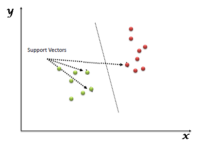
SVM_1
Support Vectors are simply the co-ordinates of individual observation. Support Vector Machine is a frontier which best segregates the two classes (hyper-plane/ line).
You can look at definition of support vectors and a few examples of its working here.

How does it work?

Above, we got accustomed to the process of segregating the two classes with a hyper-plane. Now the burning question is “How can we identify the right hyper-plane?”. Don’t worry, it’s not as hard as you think!
Let’s understand:
  • Identify the right hyper-plane (Scenario-1): Here, we have three hyper-planes (A, B and C). Now, identify the right hyper-plane to classify star and circle.
    SVM_2You need to remember a thumb rule to identify the right hyper-plane: “Select the hyper-plane which segregates the two classes better”. In this scenario, hyper-plane “B” has excellently performed this job.
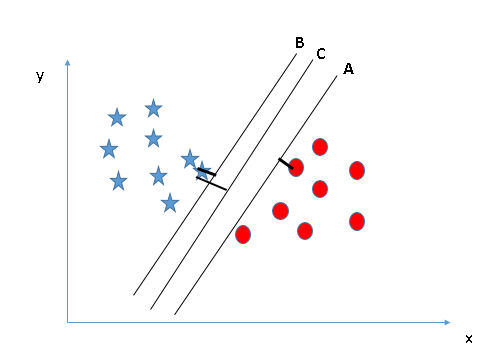
  • Identify the right hyper-plane (Scenario-2): Here, we have three hyper-planes (A, B and C) and all are segregating the classes well. Now, How can we identify the right hyper-plane?
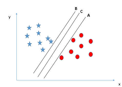
    SVM_3Here, maximizing the distances between nearest data point (either class) and hyper-plane will help us to decide the right hyper-plane. This distance is called as Margin. Let’s look at the below snapshot:SVM_4
    Above, you can see that the margin for hyper-plane C is high as compared to both A and B. Hence, we name the right hyper-plane as C. Another lightning reason for selecting the hyper-plane with higher margin is robustness. If we select a hyper-plane having low margin then there is high chance of miss-classification.
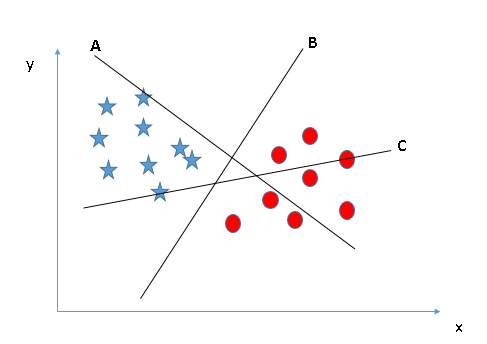
  • Identify the right hyper-plane (Scenario-3):Hint: Use the rules as discussed in previous section to identify the right hyper-plane
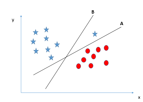
SVM_5Some of you may have selected the hyper-plane B as it has higher margin compared to A. But, here is the catch, SVM selects the hyper-plane which classifies the classes accurately prior to maximizing margin. Here, hyper-plane B has a classification error and A has classified all correctly. Therefore, the right hyper-plane is A.
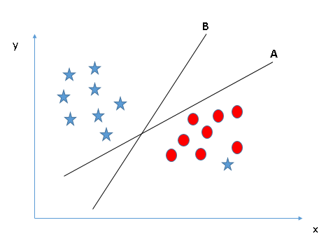
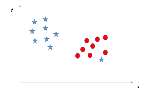
  • Can we classify two classes (Scenario-4)?: Below, I am unable to segregate the two classes using a straight line, as one of star lies in the territory of other(circle) class as an outlier. 
    SVM_6
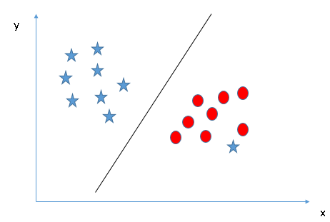
    As I have already mentioned, one star at other end is like an outlier for star class. SVM has a feature to ignore outliers and find the hyper-plane that has maximum margin. Hence, we can say, SVM is robust to outliers.
    SVM_7
  • Find the hyper-plane to segregate to classes (Scenario-5): In the scenario below, we can’t have linear hyper-plane between the two classes, so how does SVM classify these two classes? Till now, we have only looked at the linear hyper-plane.
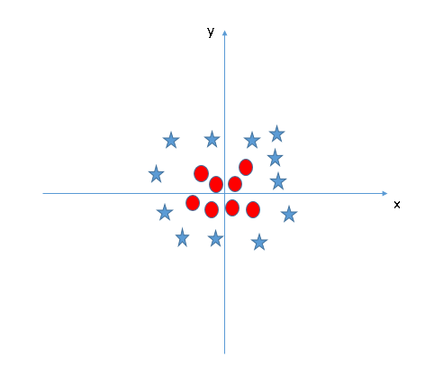
    SVM_8
    SVM can solve this problem. Easily! It solves this problem by introducing additional feature. Here, we will add a new feature z=x^2+y^2. Now, let’s plot the data points on axis x and z:
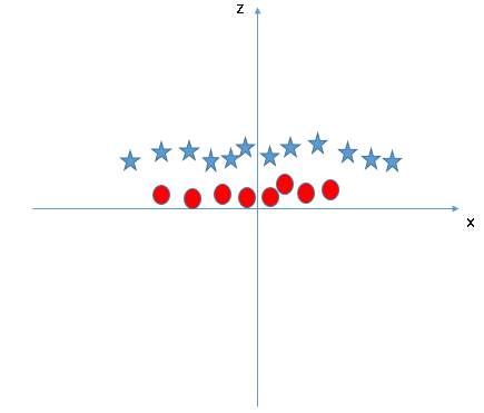
    SVM_9
    In above plot, points to consider are:
    • All values for z would be positive always because z is the squared sum of both x and y
    • In the original plot, red circles appear close to the origin of x and y axes, leading to lower value of z and star relatively away from the origin result to higher value of z.
    In SVM, it is easy to have a linear hyper-plane between these two classes. But, another burning question which arises is, should we need to add this feature manually to have a hyper-plane. No, SVM has a technique called the kernel trick. These are functions which takes low dimensional input space and transform it to a higher dimensional space i.e. it converts not separable problem to separable problem, these functions are called kernels. It is mostly useful in non-linear separation problem. Simply put, it does some extremely complex data transformations, then find out the process to separate the data based on the labels or outputs you’ve defined.
    When we look at the hyper-plane in original input space it looks like a circle:
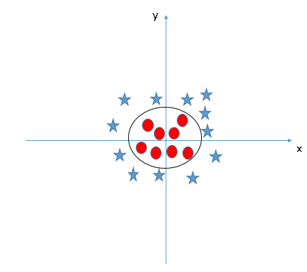
    SVM_10
Now, let’s  look at the methods to apply SVM algorithm in a data science challenge.

How to implement SVM in Python?

In Python, scikit-learn is a widely used library for implementing machine learning algorithms, SVM is also available in scikit-learn library and follow the same structure (Import library, object creation, fitting model and prediction). Let’s look at the below code:
#Import Library
from sklearn import svm
#Assumed you have, X (predictor) and Y (target) for training data set and x_test(predictor) of test_dataset
# Create SVM classification object 
model = svm.svc(kernel='linear', c=1, gamma=1) 
# there is various option associated with it, like changing kernel, gamma and C value. Will discuss more # about it in next section.Train the model using the training sets and check score
model.fit(X, y)
model.score(X, y)
#Predict Output
predicted= model.predict(x_test)

How to tune Parameters of SVM?

Tuning parameters value for machine learning algorithms effectively improves the model performance. Let’s look at the list of parameters available with SVM.
sklearn.svm.SVC(C=1.0, kernel='rbf', degree=3, gamma=0.0, coef0=0.0, shrinking=True, probability=False,tol=0.001, cache_size=200, class_weight=None, verbose=False, max_iter=-1, random_state=None)
I am going to discuss about some important parameters having higher impact on model performance, “kernel”, “gamma” and “C”.
kernel: We have already discussed about it. Here, we have various options available with kernel like, “linear”, “rbf”,”poly” and others (default value is “rbf”).  Here “rbf” and “poly” are useful for non-linear hyper-plane. Let’s look at the example, where we’ve used linear kernel on two feature of iris data set to classify their class.
Example: Have linear kernel
import numpy as np
import matplotlib.pyplot as plt
from sklearn import svm, datasets
# import some data to play with
iris = datasets.load_iris()
X = iris.data[:, :2] # we only take the first two features. We could
 # avoid this ugly slicing by using a two-dim dataset
y = iris.target
# we create an instance of SVM and fit out data. We do not scale our
# data since we want to plot the support vectors
C = 1.0 # SVM regularization parameter
svc = svm.SVC(kernel='linear', C=1,gamma=0).fit(X, y)
# create a mesh to plot in
x_min, x_max = X[:, 0].min() - 1, X[:, 0].max() + 1
y_min, y_max = X[:, 1].min() - 1, X[:, 1].max() + 1
h = (x_max / x_min)/100
xx, yy = np.meshgrid(np.arange(x_min, x_max, h),
 np.arange(y_min, y_max, h))
plt.subplot(1, 1, 1)
Z = svc.predict(np.c_[xx.ravel(), yy.ravel()])
Z = Z.reshape(xx.shape)
plt.contourf(xx, yy, Z, cmap=plt.cm.Paired, alpha=0.8)
plt.scatter(X[:, 0], X[:, 1], c=y, cmap=plt.cm.Paired)
plt.xlabel('Sepal length')
plt.ylabel('Sepal width')
plt.xlim(xx.min(), xx.max())
plt.title('SVC with linear kernel')
plt.show()SVM_11
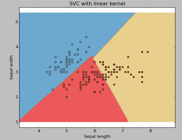
Example: Have rbf kernel
Change the kernel type to rbf in below line and look at the impact.
svc = svm.SVC(kernel='rbf', C=1,gamma=0).fit(X, y)
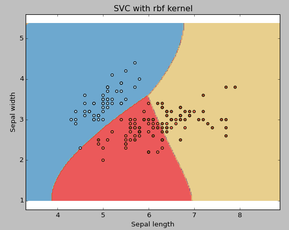
SVM_12

I would suggest you to go for linear kernel if you have large number of features (>1000) because it is more likely that the data is linearly separable in high dimensional space. Also, you can RBF but do not forget to cross validate for its parameters as to avoid over-fitting.
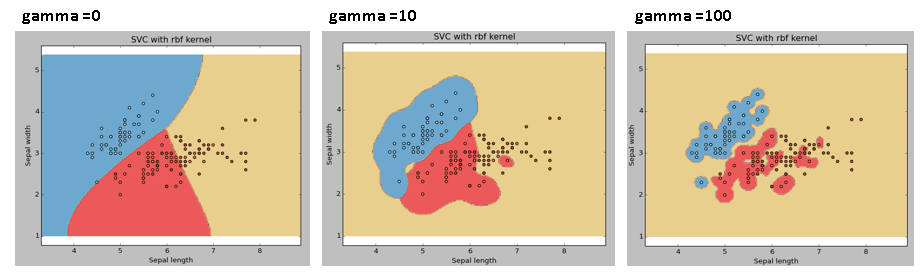
gamma: Kernel coefficient for ‘rbf’, ‘poly’ and ‘sigmoid’. Higher the value of gamma, will try to exact fit the as per training data set i.e. generalization error and cause over-fitting problem.
Example: Let’s difference if we have gamma different gamma values like 0, 10 or 100.
svc = svm.SVC(kernel='rbf', C=1,gamma=0).fit(X, y)
SVM_15
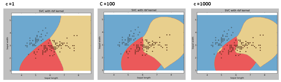
C: Penalty parameter C of the error term. It also controls the trade off between smooth decision boundary and classifying the training points correctly.
SVM_18
We should always look at the cross validation score to have effective combination of these parameters and avoid over-fitting.

Pros and Cons associated with SVM

  • Pros:
    • It works really well with clear margin of separation
    • It is effective in high dimensional spaces.
    • It is effective in cases where number of dimensions is greater than the number of samples.
    • It uses a subset of training points in the decision function (called support vectors), so it is also memory efficient.
  • Cons:
    • It doesn’t perform well, when we have large data set because the required training time is higher
    • It also doesn’t perform very well, when the data set has more noise i.e. target classes are overlapping
    • SVM doesn’t directly provide probability estimates, these are calculated using an expensive five-fold cross-validation. It is related SVC method of Python scikit-learn library.

Practice Problem

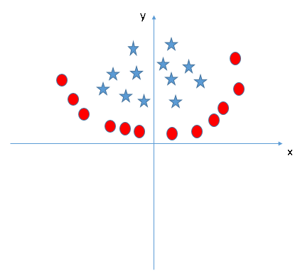
Find right additional feature to have a hyper-plane for segregating the classes in below snapshot:
SVM_19
Answer the variable name in the comments section below. I’ll shall then reveal the answer.

End Notes

In this article, we looked at the machine learning algorithm, Support Vector Machine in detail.  I discussed its concept of working, process of implementation in python, the tricks to make the model efficient by tuning its parameters, Pros and Cons, and finally a problem to solve. I would suggest you to use SVM and analyse the power of this model by tuning the parameters. I also want to hear your experience with SVM, how have you tuned parameters to avoid over-fitting and reduce the training time?
Did you find this article helpful? Please share your opinions / thoughts in the comments section below.

Recognizing hand-written digits

Source:
print(__doc__)

# Author: Gael Varoquaux <gael dot varoquaux at normalesup dot org>
# License: BSD 3 clause

# Standard scientific Python imports
import matplotlib.pyplot as plt

# Import datasets, classifiers and performance metrics
from sklearn import datasets, svm, metrics

# The digits dataset
digits = datasets.load_digits()

# The data that we are interested in is made of 8x8 images of digits, let's
# have a look at the first 4 images, stored in the `images` attribute of the
# dataset.  If we were working from image files, we could load them using
# matplotlib.pyplot.imread.  Note that each image must have the same size. For these
# images, we know which digit they represent: it is given in the 'target' of
# the dataset.
images_and_labels = list(zip(digits.images, digits.target))
for index, (image, label) in enumerate(images_and_labels[:4]):
    plt.subplot(2, 4, index + 1)
    plt.axis('off')
    plt.imshow(image, cmap=plt.cm.gray_r, interpolation='nearest')
    plt.title('Training: %i' % label)

# To apply a classifier on this data, we need to flatten the image, to
# turn the data in a (samples, feature) matrix:
n_samples = len(digits.images)
data = digits.images.reshape((n_samples, -1))

# Create a classifier: a support vector classifier
classifier = svm.SVC(gamma=0.001)

# We learn the digits on the first half of the digits
classifier.fit(data[:n_samples // 2], digits.target[:n_samples // 2])

# Now predict the value of the digit on the second half:
expected = digits.target[n_samples // 2:]
predicted = classifier.predict(data[n_samples // 2:])

print("Classification report for classifier %s:\n%s\n"
      % (classifier, metrics.classification_report(expected, predicted)))
print("Confusion matrix:\n%s" % metrics.confusion_matrix(expected, predicted))

images_and_predictions = list(zip(digits.images[n_samples // 2:], predicted))
for index, (image, prediction) in enumerate(images_and_predictions[:4]):
    plt.subplot(2, 4, index + 5)
    plt.axis('off')
    plt.imshow(image, cmap=plt.cm.gray_r, interpolation='nearest')
    plt.title('Prediction: %i' % prediction)

plt.show()
bổ sung:
để chạy được thì cần phải có 2 module:
matplotlib và tkinter

pip install matplotlib
sudo apt-get install python-tk (sd module này cho python 2)

sudo apt-get install python3-tk (sd module này cho python 3)

scikit-learn quick start

Machine learning: the problem setting

In general, a learning problem considers a set of n samples of data and then tries to predict properties of unknown data. If each sample is more than a single number and, for instance, a multi-dimensional entry (aka multivariate data), it is said to have several attributes or features.
We can separate learning problems in a few large categories:
  • supervised learning, in which the data comes with additional attributes that we want to predict (Click here to go to the scikit-learn supervised learning page).This problem can be either:
    • classification: samples belong to two or more classes and we want to learn from already labeled data how to predict the class of unlabeled data. An example of classification problem would be the handwritten digit recognition example, in which the aim is to assign each input vector to one of a finite number of discrete categories. Another way to think of classification is as a discrete (as opposed to continuous) form of supervised learning where one has a limited number of categories and for each of the n samples provided, one is to try to label them with the correct category or class.
    • regression: if the desired output consists of one or more continuous variables, then the task is called regression. An example of a regression problem would be the prediction of the length of a salmon as a function of its age and weight.
  • unsupervised learning, in which the training data consists of a set of input vectors x without any corresponding target values. The goal in such problems may be to discover groups of similar examples within the data, where it is called clustering, or to determine the distribution of data within the input space, known as density estimation, or to project the data from a high-dimensional space down to two or three dimensions for the purpose of visualization (Click here to go to the Scikit-Learn unsupervised learning page).
Training set and testing set
Machine learning is about learning some properties of a data set and applying them to new data. This is why a common practice in machine learning to evaluate an algorithm is to split the data at hand into two sets, one that we call the training set on which we learn data properties and one that we call the testing set on which we test these properties.

Loading an example dataset

scikit-learn comes with a few standard datasets, for instance the iris and digits datasets for classification and the boston house prices dataset for regression.
In the following, we start a Python interpreter from our shell and then load the iris and digits datasets. Our notational convention is that $ denotes the shell prompt while >>> denotes the Python interpreter prompt:
$ python
>>> from sklearn import datasets
>>> iris = datasets.load_iris()
>>> digits = datasets.load_digits()
A dataset is a dictionary-like object that holds all the data and some metadata about the data. This data is stored in the .data member, which is a n_samples, n_features array. In the case of supervised problem, one or more response variables are stored in the .target member. More details on the different datasets can be found in the dedicated section.
For instance, in the case of the digits dataset, digits.data gives access to the features that can be used to classify the digits samples:
>>>
>>> print(digits.data)  
[[  0.   0.   5. ...,   0.   0.   0.]
 [  0.   0.   0. ...,  10.   0.   0.]
 [  0.   0.   0. ...,  16.   9.   0.]
 ...,
 [  0.   0.   1. ...,   6.   0.   0.]
 [  0.   0.   2. ...,  12.   0.   0.]
 [  0.   0.  10. ...,  12.   1.   0.]]
and digits.target gives the ground truth for the digit dataset, that is the number corresponding to each digit image that we are trying to learn:
>>>
>>> digits.target
array([0, 1, 2, ..., 8, 9, 8])
Shape of the data arrays
The data is always a 2D array, shape (n_samples, n_features), although the original data may have had a different shape. In the case of the digits, each original sample is an image of shape (8, 8) and can be accessed using:
>>>
>>> digits.images[0]
array([[  0.,   0.,   5.,  13.,   9.,   1.,   0.,   0.],
       [  0.,   0.,  13.,  15.,  10.,  15.,   5.,   0.],
       [  0.,   3.,  15.,   2.,   0.,  11.,   8.,   0.],
       [  0.,   4.,  12.,   0.,   0.,   8.,   8.,   0.],
       [  0.,   5.,   8.,   0.,   0.,   9.,   8.,   0.],
       [  0.,   4.,  11.,   0.,   1.,  12.,   7.,   0.],
       [  0.,   2.,  14.,   5.,  10.,  12.,   0.,   0.],
       [  0.,   0.,   6.,  13.,  10.,   0.,   0.,   0.]])
The simple example on this dataset illustrates how starting from the original problem one can shape the data for consumption in scikit-learn.
Loading from external datasets
To load from an external dataset, please refer to loading external datasets.

Learning and predicting

In the case of the digits dataset, the task is to predict, given an image, which digit it represents. We are given samples of each of the 10 possible classes (the digits zero through nine) on which we fit an estimator to be able to predict the classes to which unseen samples belong.
In scikit-learn, an estimator for classification is a Python object that implements the methods fit(X, y) and predict(T).
An example of an estimator is the class sklearn.svm.SVC that implements support vector classification. The constructor of an estimator takes as arguments the parameters of the model, but for the time being, we will consider the estimator as a black box:
>>>
>>> from sklearn import svm
>>> clf = svm.SVC(gamma=0.001, C=100.)
Choosing the parameters of the model
In this example we set the value of gamma manually. It is possible to automatically find good values for the parameters by using tools such as grid search and cross validation.
We call our estimator instance clf, as it is a classifier. It now must be fitted to the model, that is, it must learn from the model. This is done by passing our training set to the fit method. As a training set, let us use all the images of our dataset apart from the last one. We select this training set with the [:-1] Python syntax, which produces a new array that contains all but the last entry of digits.data:
>>>
>>> clf.fit(digits.data[:-1], digits.target[:-1])  
SVC(C=100.0, cache_size=200, class_weight=None, coef0=0.0,
  decision_function_shape=None, degree=3, gamma=0.001, kernel='rbf',
  max_iter=-1, probability=False, random_state=None, shrinking=True,
  tol=0.001, verbose=False)
Now you can predict new values, in particular, we can ask to the classifier what is the digit of our last image in the digits dataset, which we have not used to train the classifier:
>>>
>>> clf.predict(digits.data[-1:])
array([8])
The corresponding image is the following:
../../_images/sphx_glr_plot_digits_last_image_001.png As you can see, it is a challenging task: the images are of poor resolution. Do you agree with the classifier?
A complete example of this classification problem is available as an example that you can run and study: Recognizing hand-written digits.

Model persistence

It is possible to save a model in the scikit by using Python’s built-in persistence model, namely pickle:
>>>
>>> from sklearn import svm
>>> from sklearn import datasets
>>> clf = svm.SVC()
>>> iris = datasets.load_iris()
>>> X, y = iris.data, iris.target
>>> clf.fit(X, y)  
SVC(C=1.0, cache_size=200, class_weight=None, coef0=0.0,
  decision_function_shape=None, degree=3, gamma='auto', kernel='rbf',
  max_iter=-1, probability=False, random_state=None, shrinking=True,
  tol=0.001, verbose=False)

>>> import pickle
>>> s = pickle.dumps(clf)
>>> clf2 = pickle.loads(s)
>>> clf2.predict(X[0:1])
array([0])
>>> y[0]
0
In the specific case of the scikit, it may be more interesting to use joblib’s replacement of pickle (joblib.dump & joblib.load), which is more efficient on big data, but can only pickle to the disk and not to a string:
>>>
>>> from sklearn.externals import joblib
>>> joblib.dump(clf, 'filename.pkl') 
Later you can load back the pickled model (possibly in another Python process) with:
>>>
>>> clf = joblib.load('filename.pkl') 
Note
joblib.dump and joblib.load functions also accept file-like object instead of filenames. More information on data persistence with Joblib is available here.
Note that pickle has some security and maintainability issues. Please refer to section Model persistence for more detailed information about model persistence with scikit-learn.

Conventions

scikit-learn estimators follow certain rules to make their behavior more predictive.

Type casting

Unless otherwise specified, input will be cast to float64:
>>>
>>> import numpy as np
>>> from sklearn import random_projection

>>> rng = np.random.RandomState(0)
>>> X = rng.rand(10, 2000)
>>> X = np.array(X, dtype='float32')
>>> X.dtype
dtype('float32')

>>> transformer = random_projection.GaussianRandomProjection()
>>> X_new = transformer.fit_transform(X)
>>> X_new.dtype
dtype('float64')
In this example, X is float32, which is cast to float64 by fit_transform(X).
Regression targets are cast to float64, classification targets are maintained:
>>>
>>> from sklearn import datasets
>>> from sklearn.svm import SVC
>>> iris = datasets.load_iris()
>>> clf = SVC()
>>> clf.fit(iris.data, iris.target)  
SVC(C=1.0, cache_size=200, class_weight=None, coef0=0.0,
  decision_function_shape=None, degree=3, gamma='auto', kernel='rbf',
  max_iter=-1, probability=False, random_state=None, shrinking=True,
  tol=0.001, verbose=False)

>>> list(clf.predict(iris.data[:3]))
[0, 0, 0]

>>> clf.fit(iris.data, iris.target_names[iris.target])  
SVC(C=1.0, cache_size=200, class_weight=None, coef0=0.0,
  decision_function_shape=None, degree=3, gamma='auto', kernel='rbf',
  max_iter=-1, probability=False, random_state=None, shrinking=True,
  tol=0.001, verbose=False)

>>> list(clf.predict(iris.data[:3]))  
['setosa', 'setosa', 'setosa']
Here, the first predict() returns an integer array, since iris.target (an integer array) was used in fit. The second predict() returns a string array, since iris.target_names was for fitting.

Refitting and updating parameters

Hyper-parameters of an estimator can be updated after it has been constructed via the sklearn.pipeline.Pipeline.set_params method. Calling fit() more than once will overwrite what was learned by any previous fit():
>>>
>>> import numpy as np
>>> from sklearn.svm import SVC

>>> rng = np.random.RandomState(0)
>>> X = rng.rand(100, 10)
>>> y = rng.binomial(1, 0.5, 100)
>>> X_test = rng.rand(5, 10)

>>> clf = SVC()
>>> clf.set_params(kernel='linear').fit(X, y)  
SVC(C=1.0, cache_size=200, class_weight=None, coef0=0.0,
  decision_function_shape=None, degree=3, gamma='auto', kernel='linear',
  max_iter=-1, probability=False, random_state=None, shrinking=True,
  tol=0.001, verbose=False)
>>> clf.predict(X_test)
array([1, 0, 1, 1, 0])

>>> clf.set_params(kernel='rbf').fit(X, y)  
SVC(C=1.0, cache_size=200, class_weight=None, coef0=0.0,
  decision_function_shape=None, degree=3, gamma='auto', kernel='rbf',
  max_iter=-1, probability=False, random_state=None, shrinking=True,
  tol=0.001, verbose=False)
>>> clf.predict(X_test)
array([0, 0, 0, 1, 0])
Here, the default kernel rbf is first changed to linear after the estimator has been constructed via SVC(), and changed back to rbf to refit the estimator and to make a second prediction.

Multiclass vs. multilabel fitting

When using multiclass classifiers, the learning and prediction task that is performed is dependent on the format of the target data fit upon:
>>>
>>> from sklearn.svm import SVC
>>> from sklearn.multiclass import OneVsRestClassifier
>>> from sklearn.preprocessing import LabelBinarizer

>>> X = [[1, 2], [2, 4], [4, 5], [3, 2], [3, 1]]
>>> y = [0, 0, 1, 1, 2]

>>> classif = OneVsRestClassifier(estimator=SVC(random_state=0))
>>> classif.fit(X, y).predict(X)
array([0, 0, 1, 1, 2])
In the above case, the classifier is fit on a 1d array of multiclass labels and the predict() method therefore provides corresponding multiclass predictions. It is also possible to fit upon a 2d array of binary label indicators:
>>>
>>> y = LabelBinarizer().fit_transform(y)
>>> classif.fit(X, y).predict(X)
array([[1, 0, 0],
       [1, 0, 0],
       [0, 1, 0],
       [0, 0, 0],
       [0, 0, 0]])
Here, the classifier is fit() on a 2d binary label representation of y, using the LabelBinarizer. In this case predict() returns a 2d array representing the corresponding multilabel predictions.
Note that the fourth and fifth instances returned all zeroes, indicating that they matched none of the three labels fit upon. With multilabel outputs, it is similarly possible for an instance to be assigned multiple labels:
>> from sklearn.preprocessing import MultiLabelBinarizer
>> y = [[0, 1], [0, 2], [1, 3], [0, 2, 3], [2, 4]]
>> y = preprocessing.MultiLabelBinarizer().fit_transform(y)
>> classif.fit(X, y).predict(X)
array([[1, 1, 0, 0, 0],
       [1, 0, 1, 0, 0],
       [0, 1, 0, 1, 0],
       [1, 0, 1, 1, 0],
       [0, 0, 1, 0, 1]])
In this case, the classifier is fit upon instances each assigned multiple labels. The MultiLabelBinarizer is used to binarize the 2d array of multilabels to fit upon. As a result, predict() returns a 2d array with multiple predicted labels for each instance.

vấn đề dependency của python

ubuntu luôn đi cùng với 2 bản python: python 2 và python3
vì vậy phải chú ý mặc định ubuntu đi cùng python nào (thường là 2)

trong các open source viết bằng python thìì khi import các module thì có 2 vấn đề có thể xảy ra:
1. module không có trong máy
2. build path không trỏ đến thư mục chứa module đó

giải quyết vấn đề 1: sử dụng python package index (pip):
sudo apt-get install pip
pip install tên_module

giải quyết vấn đề 2: thêm đường dẫn thư muc của module vào biến sys.path của python
$python
>>> sys.path.append('path/to/to/folder/that/contains/module')

Friday, August 4, 2017

Installing scikit-learn on linux


Scikit-learn requires:
Python (>= 2.6 or >= 3.3),
NumPy (>= 1.6.1),
SciPy (>= 0.9).

Python: often installed in build-in linux distro

You should  use pip to install Numpy and Scipy

sudo apt-get install pip
pip install Numpy
pip install Scipy
pip install -U scikit-learn

bonus: (phải tự mò ra, khổ vãi, open source thì đi cùng với vấn đề là dependency - không biết cái mã nguồn naỳ cần những cái dependency nào...)

cài pip (python package index)
sudo apt-get install pip

update pip
pip install --upgrade pip

xem vị trí các module Numpy, Scipy, scikit-learn
pip list
pip show Numpy
pip show Scipy
pip show scikit-learn

thiết lập sys.path của python trỏ đến các thư mục chứa module
$python
>>>import sys
>>>sys.path.append('path/to/the/folder/that/contains/module')

Friday, July 28, 2017

Tình hình AI tại thị trường Việt Nam – Đầy khó khăn và thách thức

Nhắc tới “artificial intelligence”, “machine learning”, hay “neural nets” với bất kì nhóm software engineers nào mà bạn gặp, tôi bảo đảm bạn sẽ nghe một đống chuyện từ họ. Trong thời đại này, tất cả các ông lớn về công nghệ đều sẵn sàng chi mạnh tay để có tích hợp những công nghệ đấy vào sản phẩm của họ. Ngay cả các software engineer mới cũng cố gắng tham gia vào mỏ vàng trên.
Artificial intelligence thực chất chính là cách ta tái tạo và mô phỏng theo trí não của con người. Mục tiêu là để cho ra đời những bộ máy có khả năng thực hiện được những công việc chỉ có con người mới làm được như là biểu đạt cảm xúc, đó không phải là một việc dễ dàng. Chính vì thế mà hôm nay, Vietcetera phỏng vấn anh Herve Vu Roussel, head of data engineering tại AI firm Sentifi– một trong những người đi đầu về AI tại Việt Nam. Cùng lắng nghe những chia sẻ, quan điểm của anh về cộng đồng và khả năng phát triển cho AI tại thị trường Việt Nam.

Tình hình phát triển AI tại Việt Nam hiện nay như thế nào?

Đây là một câu hỏi khó, bởi không như San Francisco hay Montreal, Việt Nam vẫn chưa thật sự được phát triển hết tiềm năng của nó. Chúng ta vẫn còn đang trên tiến trình phát triển. Nói đến một số cá nhân/ tổ chức nổi bật thì tôi nghĩ tới Tinypulse và Trusting Social. Tinypulse nhắm tới cải thiện tinh thần cho nhân viên và khiến họ gắn bó với công ty thông qua các khảo sát, phân tích cảm xúc, natural language processing. Trusting Social, theo tôi, là một ngôi sao đang lên. Là đối tác với Viettel, công ty vừa kêu gọi vốn thành công lên đến vài triệu đô. Ý tưởng đằng sau Trusting Social là liên quan đến việc tính toán và phỏng đoán các con số. Khá là thú vị bởi khả năng ứng dụng cho nhiều lĩnh vực khác nhau của nó.

Tôi nghĩ thì hiện tại Sentifi vẫn đang đứng đầu những công ty mạnh về AI tại Việt Nam. Chúng tôi là công ty đi tiên phong về sử dụng mảng trí tuệ nhân tạo trong non-trivial applications. Nhóm data engineering của chúng tôi sử dụng machine learning, deep learning, và AI để phân tích hơn một tỉ tweets mỗi tháng để thu được insight từ cộng đồng. Sau đó dựa vào những data đó chung tôi liên hệ với những phân tích từ thị trường tài chính. Đó là cách giải thích đơn giản nhất mà tôi có thể đưa ra. Điều làm khác biệt Sentifi với các đối thủ khác nằm ở việc các sản phẩm của hãng đều tích hợp những công nghệ đi đầu thị trường Việt Nam.
Tôi tin rằng trong tương lai không xa, AI sẽ giúp cải thiện chất lượng dịch vụ tại Việt Nam. Ví dụ như giờ bạn đã có thể khám bệnh online, có một AI chuyên theo dõi sức khỏe và chăm sóc nhắc nhở bạn hay việc gửi hình X-quang để cho phỏng đoán bệnh tình mà không hề thua kém một bác sĩ thực thụ.

Có cộng đồng AI nào lớn tại Việt Nam?

Thật không may là hiện tại vẫn chưa có. Chỉ vài nhóm nhỏ lẻ trên Facebook với tính tương tác thấp. Tháng 3 vừa rồi, IBM AI XPRIZE có tổ chức sự kiện AI đầu tiên tại Việt Nam. Với hơn trăm người tham dự. Bạn có thể nói mọi người đều rất tò mò và muốn tìm hiểu về AI nhưng phần lớn đều chưa có kinh nghiệm hay đủ trình độ để hiểu sâu về nó. Vì vậy mà chúng tôi cũng đang cố gắng thúc đẩy AI tại Việt Nam nhưng cần thêm thời gian.
Từng làm việc vài lần với AI XPRIZE cũng như hướng dẫn nhiều teams tại Việt Nam, XPRIZE là một tổ chức phi lợi nhuận chuyên khuyến khích tranh tài nhằm cải thiện kiến thức chung của thế giới. Tổ chức này cũng lên một kế hoạch phát triển AI trong vòng 4 năm nhằm giải quyết các vấn đề nan giải của nhân loại. Phần thưởng cho team thắng cuộc là 5 triệu đô và cơ hội được diễn thuyết tại TED 2020. Ngoài ra nhiều công ty và nguồn lực sẽ hộ trợ cho các nhóm tham gia XPRIZE. Tôi muốn gửi thông điệp rằng Việt Nam có tiềm năng rất lớn trong AI.
-------------------- Thông tin cho Dev --------------------

Nói về công việc của tôi với XPRIZE, tôi chủ yếu nắm vai trò hướng dẫn và giúp các team Việt Nam. Hiện các nhóm đều có cho mình những project khá thú vị. Như Altoera với ý tưởng kết hợp computer vision, hardware, và software nhằm tạo ra tính năng image recognition để phát hiện sâu bệnh của cây trồng. Hiện mọi thứ chỉ ở software nhưng trong tương lai thì chúng tôi sẽ phát triển cả robot để chúng theo dõi và diệt trừ sâu bệnh luôn. Một project khác cũng rất có triển vọng là Dropdeck, với ý tưởng kết nối các nhà đầu tư với  startup entrepreneurs và giúp bảo đảm các startup có thể tìm kiếm nguồn vốn đầu tư dễ dàng hơn.

Lời khuyên của anh đối với những bạn muốn tham gia vào lĩnh vực này?

Hãy tìm kiếm thông tin tuyển dụng của các công ty AI và vào làm cho họ. Ngoài ra hãy có những project của riêng mình cũng như tham gia một số cuộc thi trên Kaggle. Ngoài ra còn rất nhiều nguồn online với hình thức tượng tự như Coursera, gồm các khóa học từ các đại học danh tiếng trên thế giới. Không có lí gì mà bạn không thể tự học trong hời đại internet này.

Điều gì đang cản trở sự phát triển của AI tại Việt Nam?

Một trong những vấn đề lớn nhất là đầu vào quá khó. Mất 1 đến 2 năm chỉ để nghiên cứu tìm hiểu là chuyện bình thường, rồi việc thiếu hụt về sức người – không có đủ người giỏi hiểu biết về machine learning cũng như data scientists. Hơn nữa, AI còn khá mới lạ, ngay cả trên thế giới thì số lượng công ty chuyên về trí thông minh nhân tạo cũng còn khá ít, như vậy sẽ khiến chi phí cho phát triển tăng rất nhiều.
Một vấn đề nan giải khác tại Việt Nam là việc có quá ít dữ liệu và thông tin. Mà khi nói về AI thì data luôn giữ vai trò quan trọng hàng đầu. Việt Nam rất hạn chế về khoảng này. Nói chi đâu xa, khi bạn xài Google Maps, thỉnh thoảng sẽ có những đường không hề có trên map. AI thực chất chính là việc chúng ta thu thập và sử dụng data để tạo ra nó. Như vậy nếu không có dữ liệu thì AI coi như chết.

Cái nữa là việc phát triển AI vẫn chưa được ủng hộ và khuyến khích tại Việt Nam. Bởi vì do giá lao động còn thấp nên việc áp dụng AI thật sự không hiệu quả. Đơn cử như việc dùng robot bảo vệ. Chỉ tính riêng chi phí phát triển và bảo trì robot đã mắc gấp mấy chục lần việc thuê bảo vệ. Vậy AI chỉ thực sự có đất dụng võ khi người Việt mình được cải thiện về đời sống về có mức lương cao.
Tuy vậy, giờ chúng ta đã bắt đầu nghiêm túc hơn về vấn đề trí thông minh nhân tạo. Bạn có thể thấy Google đang dần trở thành một công ty về AI. Điều Việt Nam có thể làm là đẩy mạnh nhiều chương trình cho data engineering, data mining, và databases. Nhưng quan trọng nhất là tạo ra một cộng đồng và nuôi dưỡng nó. Thật may là công nghệ phát triển rất nhanh. Hồi 10 năm trước, để kiếm được việc liên quan tới AI có thể gọi là không thể bởi nó như chỉ dành cho phim ảnh viễn tưởng thôi. Nhưng giờ thì các start-up AI bắt đầu xuất hiện trên toàn thế giới.

Anh có muốn gửi lời chia sẻ gì đến các bạn đọc không?

Bởi việc AI trở nên khá hot nên nhiều startup cứ áp dụng nó một cách vô tội vạ vào mọi thứ họ có thể. Tôi mong các bạn start-up nên nhớ quan trọng nhất vẫn là sản phẩm của mình có khả năng giải quyết vấn đề thật cho khách hàng thật vẫn là điều quan trọng nhất, AI chỉ là một phương tiện giúp ta đạt được điều đó.

Techtalk via Vietcetera

Trí tuệ nhân tạo có thực sự ghê gớm?

Bài viết của Andrew Ng - Giám đốc khoa học của Baidu, đồng sáng lập Coursera.
Andrew ng
Rất nhiều lãnh đạo có hỏi tôi về khả năng thực sự của trí tuệ nhân tạo. Họ muốn có cái nhìn khách quan nhất về ảnh hưởng của AI tới hoạt động của doanh nghiệp mà họ đang nắm giữ.
Qua sách, báo, blog, truyền hình,... Các bạn đều thấy AI đang thể hiện vai trò tuyệt đối của mình trong các bài toán rất phức tạp và đa dạng trong các lĩnh vực như: tìm kiếm, quảng cáo, thương mại điện tử, tài chính,... Tuy nhiên, giới truyền thông đang tung hô và thần thánh hóa AI một cách ngoạn mục.
Tôi - Andrew Ng, cựu team lead của Google Brain, nguyên giám đốc phòng thí nghiệm AI của đại học Stanford. Tôi đã phát triển rồi dẫn dắt những team làm AI hàng đầu thế giới và cho ra các sản phẩm AI được hàng triệu người sử dụng. Tôi đã chứng kiến sức mạnh của AI. Tuy nhiên tôi khẳng định, AI không phải là điều gì đó quá kì diệu như truyền thông đang nhắc đến.
Google Brain
Bạn sẽ bất ngờ đấy. Khác với việc được tung hô như một vị thần, trên thực tế, các quá trình triển khai AI đều hướng đến mục đích chung: đưa dữ liệu đầu vào (input) A. AI sẽ sử dụng đầu vào đó để generate dữ liệu đầu ra (output) B với tốc độ nhanh nhất có thể.
Input A Output B Ứng dụng
Ảnh Nhận dạng xem có phải là mặt người không Tự động tag ảnh
Giấy vay tiền Xác nhận xem tiền vay đã được trả chưa? Đánh giá & phê duyệt các khoản vay
Quảng cảo + thông tin người dùng Người dùng có click quảng cáo hay không Chạy banner quảng cáo
Một đoạn âm thanh Transcript (lời thoại dạng text) Nhận diện giọng nói
Một câu (tiếng Anh) Câu tương đương trong ngôn ngữ khác Dịch thuật
Dữ liệu của các cảm biến (trong máy móc..) Đánh giá rủi ro Hệ thống an toàn
Camera + các cảm biến trên xe Vị trí và trạng thái của xe Ô tô tự lái
Tham khảo các khóa học lập trình online, onlab, và thực tập lập trình tại TechMaster
Việc xây dựng được các hệ thống nhận input A và cho ra output B (gọi tắt là A -> B) sẽ làm thay đổi bộ mặt của nhiều ngành. Trong giới kỹ thuật, phương pháp xây dựng các hệ thống nhận input A và cho ra output B như trên được gọi là supervised learning (tạm dịch:học máy có giám sát).
Trí tuệ của con người thừa sức xử lý được các bài toán dạng A -> B như trên, tuy nhiên máy móc thì cần một quá trình phát triển dài hơi trước khi chạm đến đẳng cấp đó. Bạn thấy đấy, chiếc máy tính đầu tiên ra đời cách đây gần 1 thế kỷ. Trong khi đó, các hệ thống AI tối tân nhất hiện nay mới chỉ giải quyết một số bài toán cụ thể như tôi đã liệt kê ở trên.Tuy nhiên các hệ thống đó không ngừng được đầu tư và cải tiến. Đại diện sáng giá nhất của AI hiện nay sử dụng deep learning (deep learning được phát triển theo hướng mô phỏng một phần cơ chế hoạt động của não người). AI được nhiều nhóm nghiên cứu tiếp cận theo các phương pháp khác nhau. Một số nhóm đã chứng minh, bằng cả lý thuyết lẫn thực tế, rằng AI rất mạnh trong việc giải quyết các bài toán trong một ngữ cảnh cụ thể. Tuy vậy, AI cần vượt qua một "bậc thang" nữa để có được những kết quả mang tính cách mạng trên nhiều lĩnh vực. Và con đường dẫn đến "bậc thang" này vẫn chưa được tìm ra.
deep learning
Khi đã nắm được AI có thể và không thể làm những việc gì, tiếp theo ta cần kết hợp nó với chiến lược phát triển. Điều này đồng nghĩa với việc bạn phải biết được thông tin mình thu thập nằm ở đâu, thu thập như thế nào và khi thu thập thông tin  thì gặp những khó khăn gì.
Nếu để ý kỹ bạn sẽ thấy một nhược điểm của tất cả các hệ thống học máy có giám sát hiện nay: chúng cần quá nhiều input để đưa ra output.
Ví dụ, để hệ thống tự động tag đúng ảnh của một người bạn của bạn, AI cần 10.000 đến 100.000 bức ảnh và một vài thẻ tag có sẵn từ trước để nhận diện bạn của bạn.
Một hệ thống nhận diện và xử lý giọng nói cần 10.000 giờ clip audio chứa đoạn transcipt dài không quá 1000 ký tự để nhận diện đoạn transcript đó khi được đọc và in nó ra màn hình.
Để AI hoạt động hoàn hảo, việc lựa chọn input A và output B phù hợp là cực kỳ quan trọng. Nghe thì có vẻ đơn giản nhưng việc lực chọn A và B một cách tối ưu đã tạo ra nhiều cuộc cách mạng trong một số ngành công nghiệp.
Cộng đồng nghiên cứu và phát triển AI tương đối "mở" - tức các framework, source code được chia sẻ không giới hạn. Tuy nhiên có 2 khó khăn mà bất kỳ cá nhân và tổ chức nào cũng gặp phải khi áp dụng AI cho bài toán của họ:
  1. Về dữ liệu: như tôi đã đề cập ở trên, chọn input và output hợp lý là một việc quan trọng. Các ý tưởng và giải pháp triển khai của các team nghiên cứu AI có thể giống nhau nhưng việc thu thập dữ liệu đúng mẫu thì không phải team nào cũng hoàn thành tốt được. Và tất nhiên thiếu dữ liệu thì các engine AI khó có thể hoàn thành nhiệm vụ được giao.
  2. Về khả năng linh hoạt của team: các engine AI không phải là mỳ ăn liền. Bạn cần tùy biến một chút để nó phù hợp với nhu cầu và bài toán mà bạn đang cần giải quyết. Và tất nhiên rồi, không phải ai cũng có thể tùy biến các engine này.
Bạn sẽ thấy rằng tự tìm hiểu về AI thú vị hơn rất nhiều so với việc chỉ nghe truyền thông tung hô nó. Tuy giúp chúng ta rất nhiều nhưng AI cũng lấy đi của chúng ta không ít. Việc hiểu được vai trò của AI trong bài toán mà chúng ta đang giải quyết sẽ mở ra một chân trời mới cho ngành tự động hóa nói riêng và cách mang công nghiệp nói chung.
 hbr